Biodiversity comprises variability between individuals of a species, among species, and among ecosystems. Therefore, biodiversity research depends mainly on three scientific disciplines: genetics, taxonomy and systematics, and ecology. All these disciplines are much older than the term biodiversity, but fundamental for the characterization of biodiversity. The present chapter cannot substitute the respective textbooks, but instead summarizes basic concepts and definitions, together with their historical and philosophical foundations.
Characterization of biodiversity is not only a scientific exercise, but a fundamental trait of humans, deeply rooted within all cultures. It might be motivated by ecological or economic dependence, religious or aesthetic empathy (Wilson 1984), or, to put it more simply, curiosity, fascination or pastime. Philosophical foundations of our perception of, and attitude towards, biodiversity are often hidden, but nevertheless determine cultural and scientific traditions. These are changing and conflicting, reflecting the complexity of life—the buzzword "biodiversity" itself being among the best examples!
Among the earliest cultural artifacts are astoundingly accurate representations of wildlife in caves (Figures 1 to 3). Though their ritual function is unclear, they are without doubt highly reliable, "proto-scientific" representations of local fauna, much more so than medieval "Bestiaria". The very early representations are restricted to wildlife, and therefore clearly represent a hunter´s background. Cultural artefacts were made from animal products, such as bones or ivory (Figure 4). While many paintings and carvings had ritual function, and were hidden away from everyday life, other early representations are realistic pictures or stone carvings of animals occurring in the area. Research combining archaeology and zoological analysis of cave paintings revealed that these were accurate documentations of the extant fauna and must be considered as early documents in the chain of evidence for ecological change in recent times.
Figures 1 to 3 are different examples of rock art from the French province of Périgord. The pictures are about 30,000 years old, and testify complete mastery of most of the graphic arts, such as engraving, sculpture, painting and drawing. (Source: Ministère Culture communcation France: http://www.culture.gouv.fr/culture/arcnat/lascaux/en/index.html.
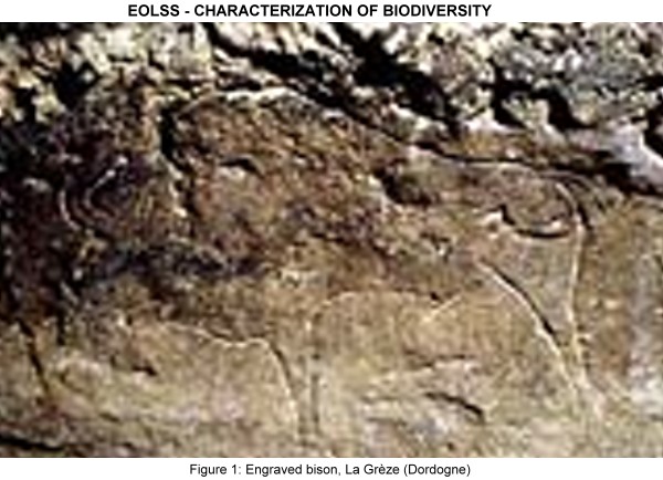
Figure 1. Engraved bison, La Grèze (Dordogne)
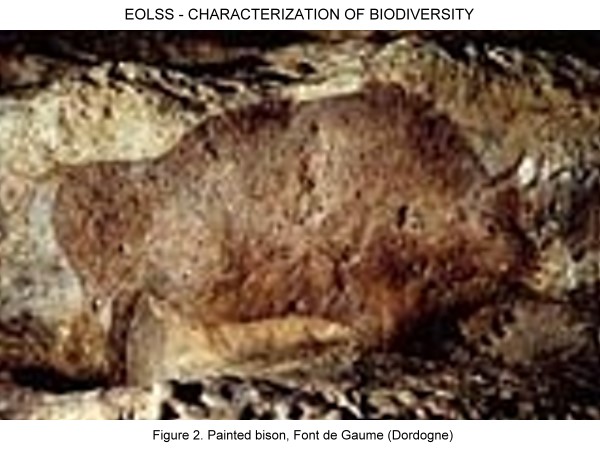
Figure 2. Painted bison, Font de Gaume (Dordogne)
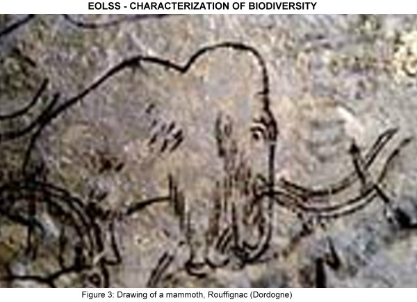
Figure 3. Drawing of a mammoth, Rouffignac (Dordogne)
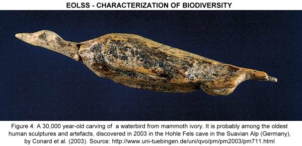
Figure 4. A 30,000 year-old carving of a waterbird from mammoth ivory. It is probably among the oldest of human sculptures and artefacts. It was discovered in 2003 in the Hohle Fels cave in the Suavian Alp (Germany), by Conard et al (2003). Source: http://www.uni-tuebingen.de/uni/qvo/pm/pm2003/pm711.html

Figure 5 . Flute from waterbird bone. Source: http://www.hr-online.de/website/fernsehen/sendungen/index.jsp?rubrik=2262& key=standard_document_1129268.
Scientific collecting is only a small part of taking of specimens, which for example includes harvesting or hunting (not only for food, but also for pleasure). All these non-scientific activities require characterization of biodiversity, often by extremely detailed terminology. Though these are not necessarily "scientific", they do reflect biological diversity reflecting species’ infraspecific variation, life-cycles or pathology. For example, hunters and fishermen have their own arcane terminology, and breeders characterize thousands of races, sports or varieties. Plant breeders require exact knowledge of cultivars, including the taxonomy and genomics of their wild relatives. Hunting, fishery and logging needs data on stocks of reliably identified species. Agriculturists must identify pest species, potential invaders and their natural enemies. In summary, all these applied fields need solid, fundamental data from biodiversity research.
A hunter’s bias prevailed until the nineteenth century, when natural history museums were filled with horns, bones, skins and feathers, and most collectors were also skilled hunters. Only in recent times did the "pursuit of the smallest game" begin, culminating in collection of thousands of insect specimens, collected by fogging rainforest trees (Figure 6). Particularly for insects, aesthetic and collectionist’s criteria such as "rarity" are a main driving force for aficionados, many of which have turned into specialists publishing scientific species descriptions.
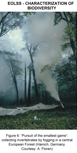
Figure 6. "Pursuit of the smallest game": collecting invertebrates by fogging in a central European Forest (Hainich, Germany. Courtesy: A. Floren)
Assigning a "name" to an observed specimen is fundamental for the description of biodiversity. Generally, such a name refers to a "species". A useful and practical definition of this intuitive process is given by Solbrig and Solbrig (1979):
We intuitively recognize a species as a group of closely similar organisms, such as humans, horses or carrots. The scientific definition has varied historically, but one that is often cited today is 'a group of morphologically similar organisms of common ancestry that under natural conditions are potentially capable of interbreeding.
However, a closer look into species definitions reveals them to be among the most difficult problems in biology. Does the name of a species reflect a man-made concept (nominalism), or does it refer to a "real" functional unit existing in nature, waiting to be discovered and named (essentialism)? This fundamental question is still discussed vigorously, though it might not always be relevant for the practitioner.
Most species definitions fall into one of three major concepts:
-
morphological species concept
-
biological species concept
-
phylogenetic species concept.
2.1. Morphological species concept
The morphological species concept has been widely used, and is also adopted in everyday life and folk taxonomies: all morphologically similar organisms have the same name (‘species’ is derived from the Latin speculare: looking). It is also known as the classical, phenetic, morphospecies and Linnean species concept. An early scientific definition goes back to Regan (1926):
"A species is a community, or a number of related communities, whose distinctive morphological characters are...sufficiently definite to entitle it, or them, to a specific name."
Modern ecological studies dealing with large samples of species-rich groups such as insects or marine invertebrates, often classify samples according to morphospecies. But it is evident that considerable morphological differences exist within species, as, for example, between different larval stages or among sexes.
2.2. Biological species concepts
Sexual dimorphism and developmental stages clearly show that a consistent species definition cannot rely on morphology alone. The following biological species concepts are based on the common notion that individuals of a species mix and reproduce:
A species is a group of interbreeding natural populations that are unable to successfully mate or reproduce with other such groups. (Dobshansky 1937; Mayr 1969).
This definition was extended by introduction of the ecological niche by Mayr 1982:
A species is a group of interbreeding natural populations unable to successfully mate or reproduce with other such groups, and which occupies a specific niche in nature."
The niche concept of a species "fitting" into "its" natural habitat is a concept appalling to our common sense and experience. However, niche concepts are themselves heavily disputed, and therefore do not necessarily clarify the issue. A biological species concept based on behaviour is known as the recognition species concept (Paterson 1985):
"A species is a group of organisms that recognize each other for the purpose of mating and fertilization".
This concept adds a behavioural component—recognition of a mate—as a prerequisite for mating and gene exchange. In fact, there are many species where elaborate signals have evolved, serving as behavioural barriers for mate finding or mating. Well-known examples are birds, frogs or grasshoppers that recognize their mates through species-specific songs. Differences in song parameters of morphologically similar cricket species have revealed their reproductive incompatibility, and led to the description of a different species based on behaviour.
There are various problems related to the biological species concept including:
-
it does not allow for parthenogenetic or vegetative reproduction,
-
hybridization between morphologically distinct ‘morphospecies’ is common in some plants, and
-
problems associated with different ‘cytotypes’ of plants.
2.3. Phylogenetic species concepts
Phylogenetic and evolutionary species concepts define species as discrete units within a continuous process of evolution. They are related by direct descendance to ancestral populations, from which they might differ now by having "changed" through mutation or genetic drift. Such an evolutionary view of species was introduced by Simpson (1951):
A species is a single lineage of ancestor-descendant populations which is distinct from other such lineages and which has its own evolutionary tendencies and historical fate.
Nixon & Wheeler (1990) define what is "distinct":
A species is the smallest aggregation of populations (sexual) or lineages (asexual) diagnosable by a unique combination of character states in comparable individuals.
Nixon and Wheeler´s definition considers the presently diagnosable species as a distinct unit (a "leaf" on an evolutionary tree). In contrast to Simpson’s definition, it does not require hypotheses about evolutionary tendency or historical fate, and therefore is more practical. But even so, any phylogenetic definition will differentiate more species than the biological definition: with the help of molecular techniques, many lineages could probably be differentiated, and considered as distinct species. In some well-known groups, such as birds and butterflies, numerous geographically separate subspecies have been described, and detailed molecular studies often reveal considerable genetic distances. Famous examples for reconstruction on ancestor-descendant populations are island species, such as the Galapagos finches (Geospiza spp.): an ancestral species from mainland South America that colonised the Galapagos, and then evolved into 13 distinct species, adapted to different ecological niches by the form of their beak. Such comparatively rapid speciation is called adaptive radiation, and is often observed on islands or isolated habitats.
Resuming, and taking into account the requirements of most practitioners, the species definition of Ehrlich and Holm (1962) recommends "reliance" on taxonomists’ views:
"A group of organisms judged by taxonomists (by diverse criteria) to be worthy of formal recognition as a distinct kind."
A closer look into both historic and actual species descriptions indicates that the majority are based on morphology. In paleontology, this is the only possibility, while recent taxonomic work on extant species often includes genetic and behavioural criteria directly related to the phylogenetic and biological species definitions. Finally, folk taxonomies must be considered as a mix, sometimes including subtle features below the species level, but often coinciding remarkably well with modern taxonomy (see Table 1).
Table 1. Variations in the correspondence between Nuaulu terminal categories and phylogenetic taxonomic ranks. Source: Ellen, 1993.
To take into account diagnosable differences within species, taxonomists accept and describe infraspecific ranks, such as subspecies, variety and form (cf. Table 2).
Table 2. A hierarchy of taxa (ranks), often characterized by defined endings, is typical for biological systematics. Ending are more consistently used in plant systematics.
Species concepts and different taxonomic opinions on the taxonomic status of closely related (sub)species clearly affect all estimates of the magnitude of biodiversity and its loss. To overcome this dilemma, conservationists defined the "Evolutionary Significant Unit" (ESU) as a group of organisms that has undergone significant genetic divergence from other populations of the same species. Identification of ESUs requires consideration of all available information, such as behaviour, distribution and results from analyzes of morphometrics, cytogenetics, allozymes and nuclear and mitochondrial DNA. ESUs are important for conservation management taking into account the precautionary principle, because a distinct population might become identified, or even evolve into, a separate species. For example, a recent study of DNA indicated a striking divergence between the western lowland gorilla (Gorilla gorilla), on the one hand, and the eastern lowland and mountain gorillas (Gorilla beringei), on the other hand (Table 3), and raised the possibility that the western and eastern populations, which are separated by about 1000 km, constitute separate species (Nowak 1999). The World Conservation Union (IUCN) now recognizes this separation into two species and 5 subspecies, some of which are at the brink of extinction.
Table 3. Old and new taxonomy of Gorilla gorilla (Savage & Wyman, 1847) (Hominidae – Primates). Source: Riede 2001.
3. Systematics
and taxonomy: classification and description
Taxonomy (gr.
tasso = to arrange) is the theory and practice of classifying and naming
objects, i.e. species in the case of biological taxonomy. The basic
process of description and naming is called alpha-taxonomy. Systematics
(gr. systematikos = ordered) is the study of the relations of organisms,
grouping them within higher units. Systematics and taxonomy are the present-day
core elements of biological classification, which can be divided into five
periods (Mayr 1969): Study of local
fauna (this includes local knowledge and non-Western folk taxonomies, as
studied by ethnobiology), Aristotle (scalae naturae), Gesner,
Adrovandus, John Ray (1627-1705), Hieronymus Bock, Linnaeus. Empirical
approach (still natural system, scalae naturae); avalanche of new species due
to expeditions, with help of indigenous people, often hunters. Darwin:
structuring groups according to common descendence. reconstruction of missing
links, primitive ancestors. Population
systematics. Present
tendencies: theories of taxonomy / systematics; nominalistic tendencies;
molecular techniques. Aristotle grouped
organisms along a scale of perfection (scalae naturae) to their degree of
perfection. Modern systematics is revealing the evolutionary relations between
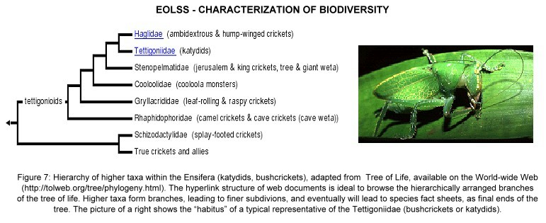
organisms, arranging them within a phylogenetic system (Figure 7). Figure 7.
Hierarchy of higher taxa within the Ensifera (katydids, bushcrickets), adapted
from Tree of Life, available on the World-wide Web
(http://tolweb.org/tree/phylogeny.html). The hyperlink structure of web
documents is ideal to browse the hierarchically arranged branches of the tree of
life. Higher taxa form branches, leading to finer subdivions, and eventually
will lead to species fact sheets, as final ends of the tree. The picture on the
right shows the "habitus" of a typical representative of the Tettigoniidae
(bushcrickets or katydids). A stringent,
methodologically elaborate theoretical framework was founded by W. Hennig and
widely disseminated by publication of the English translation of his
"phylogenetic systematics" (Hennig 1966). Hennig´s system was mainly based on
morphological features, taking the flies (Diptera) as an example. It is now
supported and complemented by genetic analysis, comparing parts of sequenced
genomes of different species, and arranging them as trees of similarity. It is
taken for granted that closer similarity is due to systematic proximity, which
means that there are "common ancestors". As result, the classification of
Biodiversity is hierarchical. Modern systematics tries to reflect the "natural"
system, based on the relation and genealogy of species as "products" of
evolution, based on Darwin´s theory and its extensions through the "modern
synthesis" (Dobshansky 1937). This natural system links species through
genealogy, and can be visualised as a "tree of life". The exact relation between
its branches is still a matter of research and discussion, even at the higher
level of the major kingdoms. The "elements" of the system are the species, which
are described and named by taxonomists. Modern taxonomic revisions not only
include (re)descriptions of related species, but also clarify their phylogenetic
position. Progress in describing and naming of species is hampered by lack of
well-trained taxonomists, especially in species-rich tropical countries, and
under-funding of "old-fashioned", "purely descriptive" taxonomy. These
shortfalls have now been identified as the "taxonomic impediment" and gave rise
to world-wide initiatives dedicated to stimulate taxonomy research, and make
their work more efficient through application of modern information technologies
(Global Biodiversity Information Facility – GBIF – http://www.gbif.org). While the higher
categories are subject to rapid changes, reflecting improved understanding of
the "true" hierarchy (descendence) of species, the alpha-taxonomic description
of individual species is regulated by rules trying to establish a certain
stability of nomenclature. Such stability is necessary for all biological
disciplines referring to certain taxa, i.e. virtually all of biology. To be
reproducible, ecological or physiological experiments must name the species (or
"model organism") used. A change of the species’ position within the tree of
life does not affect this reproducibility, while confusion due to inconsistent
or ambiguous naming of the species probably will! Besides nomenclatural
confusion, errors might arise from mis-identification. With the exception of
well-known model organims, such as rats, fruitflies or the wall cress
(Arabidopsis thaliana), these errors are frequent, and often occur in
combination. It is therefore necessary to deposit voucher specimens for later
confirmation of identification. There might even exist differences at the
infraspecific level, which might later be revealed by genetic analysis of a
properly conserved voucher specimen, or tissue sample. Up to now, there is no
regulation concerning storage of voucher specimens, which severely reduces the
value of gene databases: it is by no means clear if the species name stored in a
gene bank is correct, and based on a proper identification. Biology as a
science is unusual in that the objects of its study can be named according to
five different Codes of nomenclature. (Hawksworth 1995). Today´s
biodiversity is described through Linnean binomial nomenclature: every species
name consists of two parts, the epithet (sapiens) describing the species,
and a genus name (Homo), relating the species to a higher taxon. A
complete species name, such as Homo sapiens Linnaeus 1758, is followed by
the author and publication date of the description. In zoology, the author is
put into brackets, if the species was placed into another genus. For example,
the scientific name (generally written in italics) of the Great Egret is
Casmerodius albus (Linnaeus 1758), because it was originally described as
Egretta alba Linnaeus 1758, but subsequently moved to the genus
Casmerodius. In contrast, the scientific name of the Cocoi Heron Ardea
cocoi Linnaeus 1766 remained stable since its original description in
Linnaeus 1766. In summary, it
was Linnaeus who adopted the binomial system in his major catalogues Systema
Naturae (Linnaeus 1735) and Species Plantarum (Linnaeus 1753). Names were
followed by a diagnosis in latin, which for Homo sapiens simply consists
of the phrase "Nosce te ipsum", know yourself! Subsequently, the
Linnean binomial system evolved into frameworks of elaborate rules for naming,
called Codes. The rules governing the names of animals are laid down within the
International Code of Zoological Nomenclature (ICZN), those for naming
plants within the International Code of Botanical Nomenclature (ICBN).
Both Codes are based on the same principle: giving a unique name for each taxon.
If there are competing names, the priority rule sets that the name within
the earlier publication is valid. A third set of
rules, the Bacteriological Code, started essentially as a derivative of the ICBN
in 1953. Through a first "Approved List of Bacterial Names", it developed
into the International Code of Nomenclature of Bacteria (ICNB). During
the same period, the International Code of Nomenclature of Cultivated
Plants (ICNCP) developed and represents now a subset of rules based on the
ICBN, but adapted specifically to cultivated plants. The naming of viruses is
regulated by the International Committee on the Taxonomy of Viruses
(ICTV), which is now developing the International Code of Virus Classification
and Nomenclature, which will include sub-viral agents, such as prions. Among the
major differences between Codes are the language of the species description,
(Latin for plants, freely eligible in zoology), and the way of citing the
author. At present, most original species descriptions are not accessible and
probably not understandable for non-taxonomists. For the general
user, this diversity of Codes can cause confusion or even problems, as for
example, in the determination of which Code to follow for those organisms that
are not clearly plants, animals or bacteria, the so-called ambiregnal organisms,
or those with well-established genetic affinity, but traditional treatment as a
different group (e.g. the cyanobacteria, alias the blue-green algae. Finally,
the increasing spread of electronic retrieval systems for biological databases
confronts the user with different taxonomic concepts, or problems such as
homonymy, i.e. the same name for plants and animals. An initiative to harmonize
all biological codes resulted in attempts to draft the "BioCode" as a unified
system of biological nomenclature (Hawksworth 1995). This initiative was
discussed heavily, together with the eventual need to register names within
centralized archives. This is already the case for bacteria, where strains have
to be registered. Such an enforcement was not accepted by zoologists. Given the
high number of undescribed invertebrates, zoologists would profit from the
possibility of keeping track of the approximately 20 000 new animal names
registered each year. The inherent
insecurity of names and concepts is compensated to a certain extent by an
elaborate system of voucher specimens, which are "real-world" objects deposited
in publicly accessible collections, such as natural history museums and
herbaria. The specimen on which a description is based is called the type
specimen. A description can refer to various type specimens, and taxonomists
differentiate between holotype and paratypes, the latter
comprising a series of specimens representing the opposite sex or samples from
nearby localities. This system always allows review and eventually rewriting of
descriptions. For example, a later study might reveal that paratypes belong to
another species, or that the holotype is identical with another species, already
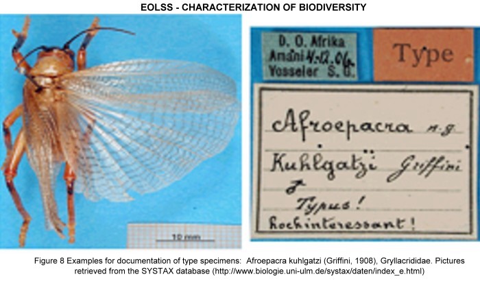
described elsewhere. Figure 8 shows an example of Orthoptera type pictures, as
published by the DORSA database. Most of the type material gathered before World
War II is deposited in US-American or European museums, reflecting the colonial
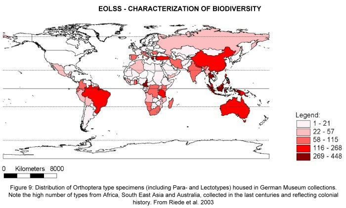
history of the respective countries. Figure 9 shows the provenance of Orthoptera
type material in German museums—the map clearly reflects the colonial history.
For plants, various parts of the same plant can be deposited in different
institutions. Figure 8. An
example of the documentation of type specimens: Afroepacra kuhlgatzi
(Griffini, 1908), Gryllacrididae. Pictures retrieved from the SYSTAX database
(http://www.biologie.uni-ulm.de/systax/daten/index_e.html) Figure 9.
Distribution of Orthoptera type specimens, housed in German Museum collections.
The legend indicates colour coding for numbers of type specimens (including
Para- and Lectotypes) per country of origin.Note the high number of types from Africa, South
East Asia and Australia, collected in the last centuries and reflecting colonial
history.
Data-basing of Natural History Collections provides access to a huge archive of information on (historical) distribution and taxonomy of organisms. This includes type specimens, which are reference objects for descriptions (names), and therefore are pivotal for linking species names (concepts) with the organismic world (objects or specimens in natural history collections). The fundamental difference between "name" and "object" information systems (taxonomic authority file databases vs specimen databases) leads to considerable friction and confusion, limiting the value of both for users who ask seemingly simple questions such as what is this species, where does it live, etc. There is a considerable number of other highly evolved databases relevant for biodiversity research, and these include information about genomes. Therefore, a complete biodiversity information infrastructure must include links to genome and protein-sequence databases. The connection is through the voucher specimens, which were hitherto not adequately referenced.
Globally, around 1.75 million species have been described and formally named to date, and there are good grounds for believing that several million more species exist but remain undiscovered and undescribed (Table 4).
Estimated numbers of described species, and possible global total.
Source: UNEP-WCMC, adapted from tables 3.1-1 and 3.1-2 of the Global Biodiversity Assessment (Heywood 1995)
The `described species' column refers to species named by taxonomists. These estimates are inevitably incomplete, because new species will have been described since publication of any checklist and more are continually being described; most groups of organisms lack a list of species and numbers are even more approximate. Most animal species, including around 8 million of the more than 10 million animal species estimated to exist, are insects. Almost 10,000 bird species and 4,640 mammals are recognized, and probably very few of either group remain to be discovered. The `estimated total' column includes provisional working estimates of described species plus the number of unknown and undescribed species; the overall estimated total figure may be highly inaccurate.
A diversity index is a mathematical measure of species diversity in a community. Diversity indices provide more information about community composition than simply species richness (i.e. the number of species present). They also take the relative abundances of different species into account. Alpha diversity refers to the diversity within a particular area or ecosystem. Table 5 summarizes indices for alpha-Diversity (a ).
Table 5. Summary of distinct diversity indices, as used in ecology.
pi = ni / N: relative abundance of a species
N = number of individuals ni = number of individuals of species i
S= total number of species
Indices for beta, and gamma diversity have been developed to measure and compare biodiversity over spatial scales (Table 6). For example, beta diversity between woodland and hedgerow habitats could be indicated by the distinct number of bird species. Gamma diversity is a measure of the overall diversity for the different ecosystems within a region.
Table 6. Indices for beta-Diversity (b ). For references, see Table 5.
Because biodiversity includes ecosystems and within-species variability, its characterization is not an exclusive domain of taxonomists. Geneticists study variability within species, and increasingly use the numerous new methodologies of DNA sequencing and fishing with DNA-probes for rapid diversity assessment of entire communities (but see Cannon 1997). To understand functional biodiversity, ecologists rely on classification of functional units ("predators") and/or life forms ("herbs"). In addition, functional units can be described and identified on the genetic level, and across species—basic ecological processes, such as photosynthesis, respiration or denitrification, are controlled by gene complexes which are homologous or analogous among a wide variety of species. Therefore, the following two sections describe characterization of biodiversity beyond the species level
6. Characterization of genetic diversity
The ample definition of biodiversity includes within-species diversity. The morphological and behavioural variability observed among individuals is the phenotype, which results from the interaction of genes—the genotype—with the environment during development. The genes are the functional units coding proteins, many of which are enzymes with vital functions for basic physiological processes. Regulatory genes control entire processes, such as development. Alleles are the different states of the same gene, coding for variations in the phenotype, such as eye colour. However, genetic differences are not necessarily diagnosed morphologically. Nevertheless, they exist and can be detected by in-depth studies of the individual’s morphology, behaviour, physiology, or by direct genetic analysis. The influence on individuals’ fitness of morphologically undetectable genetic variants or mutations can be considerable, and can even give rise to speciation. It is a common notion of present-day evolutionary theory that chance mutations are the only source of innovation during evolutionary processes. Some theoreticians consider the gene as the unit of selection ("The extended phenotype"—Dawkins 1999). Understanding genetic diversity and the underlying processes are fundamental for population genetics and population biology. In conservation biology, advanced methods such as Population Viability Analysis (PVA) quantifies "genetic erosion", which describes impoverishment of the gene pool as a consequence of population reduction and fragmentation of threatened species.
Even genetic diversity was considered by early man, who managed to breed cultivars, such as wheat and rice, by selection and farming over generations, but without the necessary scientific foundations of genetics! Evidently, there was an intuitive knowledge about heritability, and an intimate knowledge of the respective organisms, from ancestors of cultivated plants to domesticated animals (husbandry) or ornamental races. Today, the species barrier is overcome by transfer of genetic material between species, creating transgenic organisms (Table 7) through genetic engineering.
Table 7. A selection of genetically modified living organisms. Source: Global Biodiversity Outlook
The more radical forms of genetic engineering were only developed during the 1990s but already have had considerable social impact. The techniques may have great potential to improve efficiency, volume or quality in agricultural and other production processes, and these potential benefits could be of particular value to countries at risk of food insecurity. However, they also raise significant ethical and practical concerns, which have been expressed by scientists and by public opinion in both developed and developing countries.
Genetic diversity refers to any variation in the nucleotides, genes, chromosomes, or whole genomes of organisms. within the genepool of a species. The gene pool of a species or a population is the complete set of unique alleles that would be found by inspecting the genetic material of every living member of that species or population. A large gene pool indicates a large genetic diversity, which is associated with robust populations that can survive catastrophes.
The characterization of genetic diversity is intimately linked with standardized genetic techniques, which allowed comparative studies of genetic variability. Chromosomes were discovered by traditional light microscopy around the 1920s, and identified as carrier of genes (Figure 10). Cytogenetics allowed differentiation of cryptospecies and cytotypes, and in the case of giant chromosomes impressive visualisations of the genome at an astoundingly high resolution.
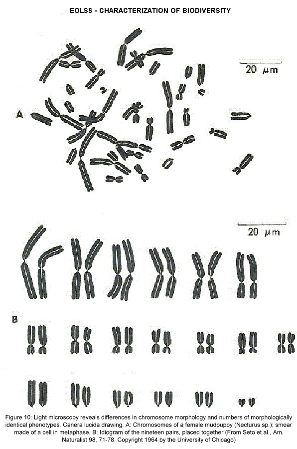
Figure 10. Light microscopy reveals differences in chromosome morphology and numbers of morphologically identical phenotypes. Canera lucida drawing. A: Chromosomes of a female mudpuppy (Necturus sp.); smear made of a cell in metaphase. B: Idiogram of the nineteen pairs, placed together. (From Seto et al., Am. Naturalist 98, 71-78. Copyright 1964 by the University of Chicago).
Chromosomal polymorphism must not lead to speciation: within the same species, forms with different chromosome numbers coexist. In most cases of polyploidy, multiples of a basic chromosome number are observed. Examples can be found among numerous plants, but also insects and fishes. As a rule, the percentage of polyploid forms seems to increase towards temperate latitudes. In some insects, such as the curculionid beetle Otiorhynchus, polyploidy is associated with parthenogenesis. In plants, the percentage of polyploids increases with altitude and towards temperate latitudes (see Table 8). Polyploidism seems to improve adaptation to extreme ecological conditions.
Table 8. Proportion of polyploids within various floras (after Margalef 1995, p. 283)
A certain "superiority" of genetically richer polyploid forms is also indicated by the fact that invasive plant species are often polyploid outside their native area, while diploid within their area of origin (e.g. the polyploid cosmopolitan invasive form of the weed Capsella bursa-pastoris, which is diploid in its Mediterranean and Armenian area of origin). In cultivars, wheat forms with higher chromosome number (14, 28 and 42, respectively), are cultivated at increasing latitudes.
Polyploidy can be generated by hybridisation among species (allopolyploidy), generating advantages due to heterosis. The increase of DNA associated with polyploidy can also be generated by endomitosis, which increases the size of the nucleus, but not the number of chromosomes.
The processes described here can be observed and characterized by light microscopy. They have been described decades ago, and include widespread genetic processes which evidently are decisive for evolution, adaptation and speciation. Nevertheless, their exact function and role is not yet understood, possibly because mainstream research concentrates on the molecular organisation of the genome. However, the significance of these processes, as summarised in Table 9, is underlined by the fact that they are under genetic control.
Table 9. Examples for regulation of gene distribution and variation
Genetic relationships between species have been analyzed by comparing polytene chromosome banding patterns, revealing patterns of fruitfly (Drosophila) speciation on Hawaiian Islands. In mosquitos (Chironomidae), banding patterns of giant chromosomes revealed clearly distinguishable differences between morphologically similar, cryptic species.
Analogous to species diversity, genetic diversity is differently patterned within and among regions and biomes. As in speciation, climate change, continental drift and geographic isolation are the main factors inducing genetic diversity. The factors inducing speciation—which means incompatibilty of genetic variants—are still mysterious: some species exhibit genetic variation over wide geographic ranges (superspecies, species rings); others develop geographically circumscribed species. Such vicariant species are evidently closely related, but "good" species. They sometimes interbreed within hybrid zones, producing more or less fertile offspring.
Among the early indicators of genetic variability were assays of enzyme variability. It is now known that this diversity is always caused by nucleotide variation within the genome. Singular nucleotide variations are mutations, which often cause lethal mis-function. Functional variants can be stabilized within the gene pool, and are characterized as distinct alleles of a certain genetic locus, or gene position within a chromosome. Genetically variable loci are polymorphic. During sexual reproduction, alleles are combined by mixing of parental chromosomes. Each parental chromosome codes for the same allele at a given locus. In general, a single letter, such as A or a, specifies the genotype of the whole chromosome with regard to the locus. An individuum with two distinct alleles is heterozygous (Aa). If one allele is recessive (symbolized by a small letter a) the morphological effect is invisible, because the phenotype is under entire control of the dominant allele (A). The independent assortment of distinct characters are called Mendelian characters. Gregor Mendel (1822 - 1884) described the laws of inheritance without knowing about genes: crossing varieties of garden peas, he considered factors of a pair of characters segregating and members of different pairs of factors assorting independently. Because chromosomes of sexually reproducing eukaryotes occur in pairs, so do the genes they contain; because homologous chromosome segments segregate during meiosis, so do the members of each pair of genes they contain.
Only the members of gene pairs located in different chromosome pairs segregate independently of each other during meiosis. Therefore, observing the inheritance of two genetically controlled phenotypes under genetic control provides evidence if the respective genes are located at distinct chromosomes. In snapdragon (Antirrhinum majus), red flowers are due to RR, white to rr, and pink to Rr; narrow leaves due to NN, broad to nn. Crossing two pink mediums (RrNn X RrNn), nine phenotypes are generated, occurring in a ratio of the expected genotypic ration due to genetic recombination of Mendelian characters (Table 10)
Table 10. Inheritance of flower colour and leave form in snapdragon (Antirrhinum majus)
In many higher organisms, one sex has XX and the other XY sex chromosomes. Several sex-linked loci are restricted to one type of sex chromosome, and, consequently, X-limited or Y-limited, as for example human colour-blindness.
Mapping the genome – linkage maps
There is cytological and genetical evidence that genetic recombination can take place within a heterozygous individual, during meiosis and/or mitosis. The consequences of such crossovers for the recombination of characters are illustrated in Figure 11. It is evident that the greater the distance between the two loci, the greater the chance for a crossing over to occur. By definition, a crossover unit is that distance between linked genes which results in 1 crossover per 100 postmeiotic products. Because the physical arrangement of loci and crossover frequencies are correlated, they can be used to construct a linear genetic map. For example, in Drosophila the arrangement of three X-limited loci – y (yellow body colour), w (white eyes), and spl (split bristles) - can be determined from crossover data, equating crossover units with map units. Note that crossover data are based on phenotypic assessment of progeny during breeding experiments. Such genetically detected crossovers are in a one-to-one correspondence with recombinant chromosomes. There is cytological evidence that crossover maps are equivalent to physical chromosome maps, because crossover frequencies are positively correlated with the frequency of chiasmata seen during meiosis. Incomplete linkage maps are available for genes in man, mouse, maize and Neurospora. They formed the starting point for the complete mapping of the genome, which was only possible by decentralized sequencing of distinct regions of the genome, which then had to be combined according to the available linkage maps.
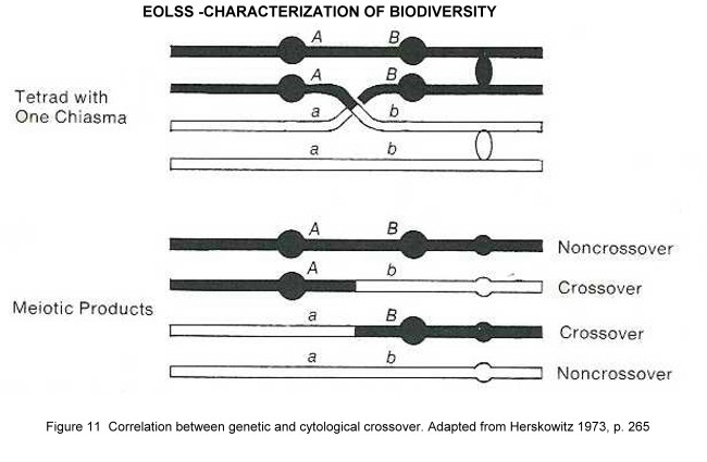
Figure 11. Correlation between genetic and cytological crossover. Adapted from Herskowitz 1973.
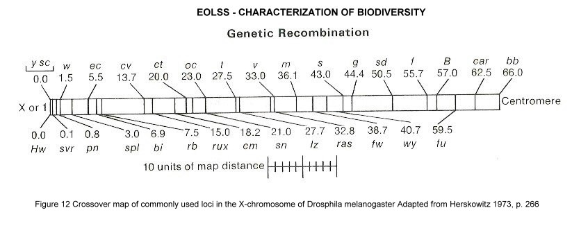
Figure 12. Crossover map of commonly used loci in the X-chromosome of Drosphila melanogaster Adapted from Herskowitz 1973.
Chromosome maps prepared by linkage models are called genetic maps. They have been prepared for many eukaryotes, including corn, Drosophila, the mouse, and the tomato.
DNA-DNA hybridization measures the degree of genetic similarity between complete genomes by measuring the amount of heat required to melt the hydrogen bonds between the base pairs that form the links between the two strands of the double helix of duplex DNA. Figure 13 shows the comparison of genetic relationship between two species A and B, by splitting and re-hybridizing their DNA. The comparison may be between the two DNA strands of an individual or of different individuals representing different levels of genetic and taxonomic divergence. The difference is a measure of genetic distance. It has been used extensively in birds (e.g. by Sibley and Monroe), revealing astounding insights into their phylogeny.
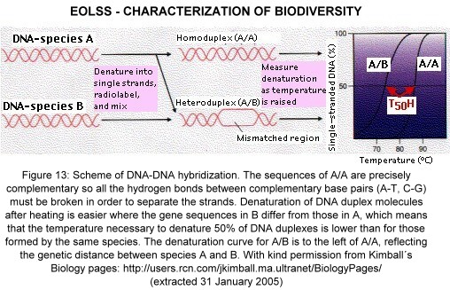
Figure 13. Scheme of DNA-DNA hybridization. The sequences of A/A are precisely complementary so all the hydrogen bonds between complementary base pairs (A-T, C-G) must be broken in order to separate the strands. Denaturation of DNA duplex molecules after heating is easier where the gene sequences in B differ from those in A, which means that the temperature necessary to denature 50% of DNA duplexes (T50H) is lower than for those formed by the same species. The denaturation curve for A/B is to the left of A/A, reflecting the genetic distance between species A and B. With kind permission from Kimball´s Biology pages: http://users.rcn.com/jkimball.ma.ultranet/BiologyPages
As an example for application of this technique, the relations between hominids are shown in Figure 14. The T50H difference between the common chimpanzee (Pan troglodytes) and the pygmy chimpanzee or bonobo (Pan paniscus) is 0.7. Assuming that their DNA has evolved at the same rate since they diverged, each branch is given one-half that value. The difference between the T50H values of humans and the chimpanzees is about 1.7, whereas that between the chimpanzees and the gorilla is 2.3. This indicates that humans and chimpanzees have shared a common ancestor more recently than chimpanzees and gorillas have. The time scale was calibrated using fossil evidence that the line to the orangutan diverged some 13–16 million years ago.

Figure 14. Phylogenetic tree of living hominoids is based on DNA-DNA hybridization data (the work of Charles Sibley and Jon Ahlquist at Yale University. With kind permission from Kimball´s Biology pages: http://users.rcn.com/jkimball.ma.ultranet/BiologyPages
Sequencing the genome
Genetic variability is visualised as tree or dendrogram of sequence similarity. Diversity is due to mutation events at nucleotide levels, and increases with unrelatedness. Divergence increases with time, and can be calibrated to a certain extent by 'molecular clocks'. Dendrograms can be produced by a wide variety of programs (e.g. Phylogenetic Analysis Using Parsimony - PAUP, see http://paup.csit.fsu.edu/), and are mainly used to reconstruct phylogenies. Sequencing of mitochondrial DNA (mtDNA) has led the way in constructing phylogenies of a wide variety of species. Other commonly used sequences are those from chloroplasts (cp) in plants, and non-coding nuclear (nc) regions in both animals and plants. MtDNA nucleotide mutation rates are fast, and appropriate for analyzing divergence within the last few million years, while those of cpDNA and ntDNA are an order of magnitude lower and therefore reflect deeper phylogenetic events. More recent events, covering periods of some 10,000 years, can be analyzed through highly variable markers, such as microsatellites and Amplified fragment length polymorphic (AFLP) markers. They reveal population variability, but are not appropriate to reveal "true" species genealogies. Population histories and their genetic variability can be analyzed efficiently through single nucleotide polymorphisms (SNPs). For a reliable reconstruction of speciation, sequence data from several independent loci should be combined.
Now that the nucleotides of the human genome have been sequenced, and the genome of the chimpanzee is nearly known, relations between hominids as shown in Figure 14 could be corroborated by direct comparisons (IHGSC 2001). There is a 98.8% coincidence between the genomes of Homo sapiens and the chimp (Pan paniscus)—the coincidence between any two humans is closer to 99.9%. Comparing over 7000 genes that occur in both species (as well as in the mouse), it turns out that slightly over 1500 of these have evolved quite differently in the two species. In humans, genes for hearing, speech and olfaction—among others—have evolved rapidly since the two species diverged, while in chimps, genes involved in formation of muscle and skeleton have evolved more rapidly.
Genetics provides the foundations for understanding generation of genetic incompatibility between species, and maintenance of diversity among their populations. H. de Vries rediscovered Mendelian principles in 1900, and T.H. Morgan developed gene theory and discovered the principle of linkage as early as 1910. It took decades from the identificiation of a ‘transforming principle’ (F. Griffith 1928), until the demonstration that this ‘principle’ is DNA by O. Avery, C. MacLeod and M. McCarthy in 1944. From there on, the rise of modern genetics led from unravelling the genetic code (Watson and Crick 1953) to the nucleotide sequencing of entire species (an animated educational module representing the timeline and milestones in genetics is available at http://www.genome.gov/Pages/EducationKit/).
7. Ecological and functional characterization of biodiversity
Ecological studies need to characterize biodiversity on higher levels. For a better understanding of interactions within a community, or entire processes (e.g. nitrogen fixation, photosynthesis), groups of species are summarized as functional types, which are defined by their inherent organismal properties related to species interactions and resources. Famous examples for functionally analogous species are the convergences observed across biogeographic realms, e.g. between marsupial and placental mammals (Figure 15). For plants, elaborate systems of vegetation classification have been developed (see below).
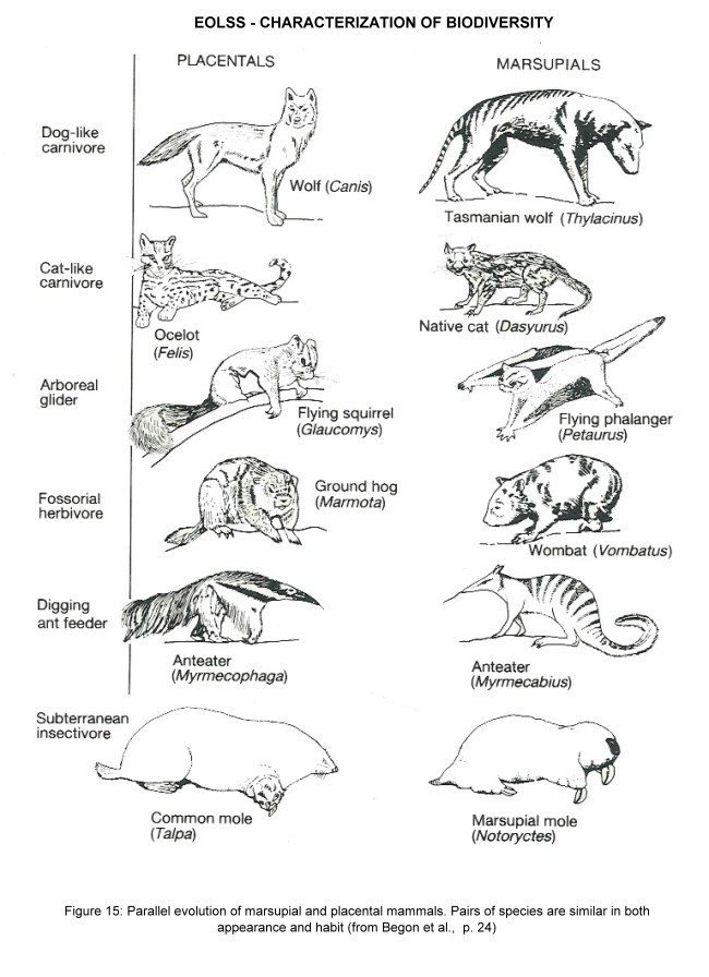
Figure 15. Parallel evolution of marsupial and placental mammals. Pairs of species are similar in both appearance and habit (from Begon et al, p. 24)
An interesting case is corals (Cnidaria: Anthozoa). Their life forms can be defined according to their architecture, forming huge construction modules of limestone skeletons, deposited by countless generations of coral polyps, which form the substance of the coral reef. The emerging complex ecosystems equal tropical rainforests in complexity and diversity. Reef structures might be compared to trees, forming the matrix of architectural complexity. In addition, polyps exhibit multiple life history strategies. Growth is mainly from asexual reproduction of colonies. But there is sexual reproduction with mobile gametes and polyps, dispersed by ocean currents, and then attaching again to a substrate, to form colonies elsewhere. In addition, corals are excellent examples for symbiosis, formed between the polyps and symbiotic algae (zooxanthellae), living and photosynthesizing within the tissues of the polyp.
On a global scale, regional classifications based on biodiversity are biogeographic zones, biomes, ecoregions and oceanic realms, subdivided into landscapes, ecoystems, communities and assemblages.
Classification systems of ecological communities can be based on the respective ecosystems or species composition (Table 11). There are no clear criteria for defining ecological units. Consequently, classifications of ecological associations are abstractions, following distinct concepts and research approaches. Clements (1919) regarded an association as a complex organism, while Gleason (1926) proposed the individualistic concept of the plant association. The boundaries between ecological units based on different concepts are necessarily arbitrary, and present serious problems of scale.
Table 11. Global classification systems: zoogeographic and floristic regions.
Adapted from Heywood 1995, p. 97.
The geographic distribution of species on earth is uneven: tropical diversity is admired since the spectacular reports of early explorers, and continues to generate headlines since the spectacular estimates of 30 million species on Earth, based on T. Erwin´s fogging experiments in Neotropical rainforests. On the other hand, temperate or even polar ecosystems are famous for their seasonal abundance and high productivity, resulting in simple foodchains culminating in high densities of charismatic ‘flagship’ species such as penguins, seals or—in historic times—whales. Whole economies were based on bounties of marine productivity, such as whales, cod or herring. Over-exploitation led to the extinction even of abundant species. Together with logging and clearing for agriculture, entire ecosystems have been totally transformed since prehistoric times. Most habitat classifications, including the map shown in Figure 16, are based on classifications of natural habitats such as would occur without human interference or might re-emerge after human intervention ceases. For instance, Central Europe is indicated on these maps as "broad-leaved temperate forest", i.e. the natural vegetation type and not the type that currently predominates (agricultural steppe, forest plantations). Most regions are severely modified, in the best of cases transformed into agro-ecosystems which at least partially mimic the original ecosystem functionality. Chapin III et al (2000) review the multiple effects of human activity on biodiversity. On a global scale, humans have transformed 40-50% of the ice-free land surface, changing prairies, forests and wetlands into agricultural and urban systems. We dominate (directly or indirectly) about one-third of the net primary productivity on land and harvest fish that use 8% of ocean productivity. We use 54% of the available fresh water, with use projected to increase to 70% by 2050. It is clear that these activities have profound effects on species numbers, but exact predictions are difficult to make. If we want to maintain species outside protected areas, or the few remaining wilderness areas, it is decisive to know the exact distribution and nature of land use. Relevant geodata layers are already available, and include population density and change rates, agriculturally used land, road density or livestock density. The FAO’s Environment and Natural Resources Service (SDRN) carries out a number of activities concerning land cover and land use, most of which apply modern techniques of remote sensing and GIS technology. Examples are the Africover Interpretation and Mapping System, or the development of a Land Cover Classification System (see http://www.fao.org/sd/eidirect/Eire0057.htm). Systematic integration of these data sets into species conservation schemes is still in its infancy.
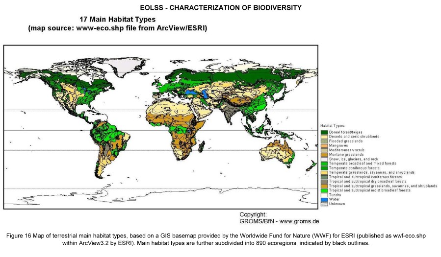
Figure 16. Map of terrestrial main habitat types, based on a GIS basemap provided by the Worldwide Fund for Nature (WWF) for ESRI (published as wwf-eco.shp within ArcView3.2 by ESRI). Main habitat types are further subdivided into 890 ecoregions, indicated by black outlines.
Description of vegetation
Physiognomy includes aspects of plant architecture, appearance of the vegetation and phenology (timing of events in a community, e.g. seasonal cycles), as well as composition of a community, mainly consisting of a plant species list, ordered according to their abundance
In Europe, during the 1930s, the Swiss ecologist Josias Braun-Blanquet (1884 – 1980) developed a method of classifying vegetation into discreet units, which he called associations. This method was based on his authoritative textbook Pflanzensoziologie (Braun-Blanquet 1928), and became the central concept of the Zürich-Montpellier School of Phytosociology. It gained wide acceptance throughout Europe, while in North America, no single classification method developed. However, the American botanist and ecologist Frederic Edward Clements (1874 – 1945) maintained that plant communities may be regarded as superorganisms. In his Research Methods in Ecology (Clements 1905) he investigated succession and development of communities into climax communities, and recognized discreet units by naming regional formations and associations. His "organismic" view of plant associations, showing "birth" and "death" during succession, was heavily critisized by later ecologists. On the other hand, his organismic view was revived to a certain extent by the Gaia hypothesis, which proposes that the earth is one large superorganism maintaining an environment suitable for life (Lovelock 2003).
Clement´s view was disputed and replaced by the individualistic hypothesis developed by Henry Gleason from 1926 until the late 1940s. He stressed the importance of species over community aspects. This importance of the floristic composition of the communities was the starting point for the continuum approach developed by John Curtis and Robert Whittaker. Whittaker studied vegetation along continuous elevation gradients in different areas of the USA. In his Classification of Plant Communities, Whittaker (1978) summarized approaches from many schools. Modern ecological studies recognize the roles of both views. Association views are somewhat subjective, but useful for communicating about vegetation, and mapping its variation. The continuum view is needed to study the response of vegetation along environmental gradients.
Besides through species composition, a plant community can be characterized by its physiognomy, which includes aspects of the plant architecture and the general appearance of the vegetation. Most vegetation analyses include only larger growth forms, using classifications of life forms. Table 12 lists classifications of some specialized plant life forms. Figure 17 shows Dansereau’s "lollipop diagrams", representing well-known vegetation forms by schematic symbols.
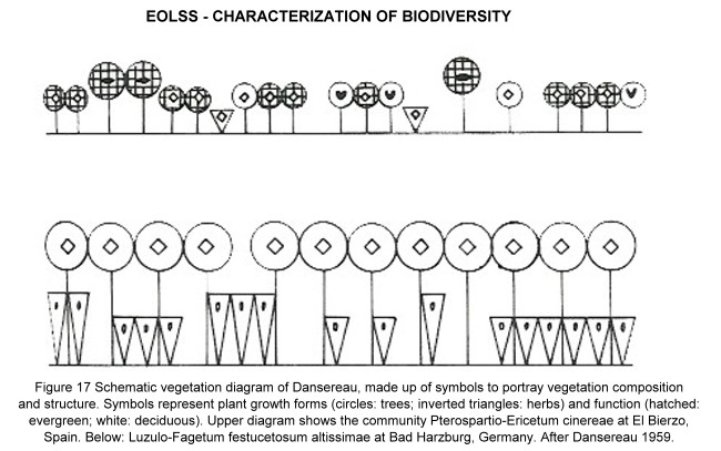
Figure 17. Schematic vegetation diagram of Dansereau, made up of symbols to portray vegetation composition and structure. Symbols represent plant growth forms (circles: trees; inverted triangles: herbs) and function (hatched: evergreen; white: deciduous). Upper diagram shows the community Pterospartio-Ericetum cinereae at El Bierzo, Spain.
Below: Luzulo-Fagetum festucetosum altissimae at Bad Harzburg, Germany. After Dansereau 1959.
Table 12. Examples for specialised life forms which are not classified on the basis of their perennating organs (adapted from Allaby 1998)
Other classifications are less intuitive, but emphasize important functional and ecological properties. A Danish ecologist, Christen Raunkiaer (1876-1960), suggested that plants evolved under tropical conditions, and then developed adaptations to survive in less hospitable areas. Consequently, he proposed a classification of plants based on the position of these perennating organs in relation to the soil surface. This classification is known as Raunkiaer's Life Forms. The classification by Raunkiaer is shown in Figure 18 (after Hickey and King 2000).
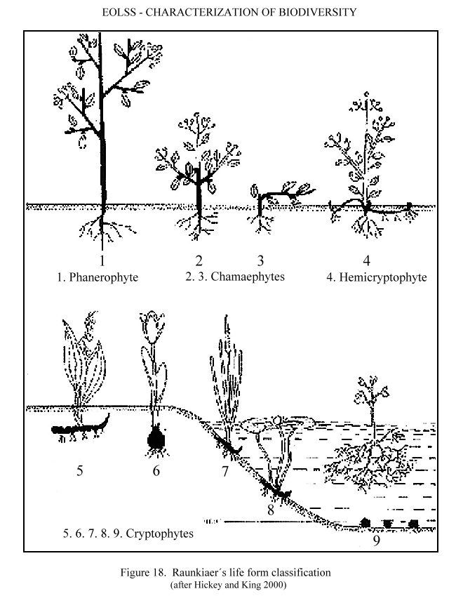
Figure 18. Raunkiaer´s life form classification (after Hickey and King 2000)
The Raunkiaer system differentiates
-
Phanerophytes
(1): A tall, woody or herbaceous perennial with resting buds more than 25cms
above soil level, e.g. deciduous trees and shrubs.